Overview
I have recently completed my Honours project in Computer Science at the University of Western Australia. My topic was “Investigating the feasibility of developing a near real-time system for music transcription on mobile devices”. On this page you will find various resources relating to this project, including software which you are free to download and run on your home computer which is capable of converting an audio signal into an abstract XML form, which can then be used for notating the music.
Software downloads
The system that was developed is available here for download.
Please note that a recent version of Java must be installed on your computer. I have only tested this under Windows and Fedora Linux; your performance may vary. If you are having problems, feel free to contact me, and I’ll try and help you resolve them. Unfortunately I cannot guarantee this software’s performance.
Notes about the application:
- It has only been tested with 16bit Mono PCM wave files sampled at 44.1kHz; it should work at other bitrates and sampling rates, but stereo/quad/etc. may not work.
- While it is working, the application may stop responding. This is normal, and the duration of this is directly proportional to the length of the signal you are transcribing. You may also notice system performance degradation during the transcription process; this is because the system uses whatever resources it can possibly get from the operating system to finish as quickly as possible.
- The system was developed using a beta version of the Java Development Kit, and a beta version of Netbeans, so these may well introduce stability issues into it, in addition to the undoubtedly very large number of bugs already in the system.
Note that this software is NOT open source and it is COPYRIGHT by me, Barry van Oudtshoorn. It is illegal to reverse engineer, distribute, copy, profit from, or otherwise steal this software. You are, however, free to use it for your own personal use, and you can even use it to help you write songs which you can sell. Basically, you can’t claim credit for the software, and you can’t sell it or distribute it without my permission.
Thesis downloads
My thesis is also available for download in PDF format. This details everything about the project, including the motivation, previous work in the area, the system’s structure, experiments performed, their results, and future work.
The thesis was typeset using LaTeX and a variety of packags, including hyperref. To follow a reference or index entry, simply click on it. The red and green boxes which indicate these hyperlinks will not be printed.
Please note that this thesis is copyright by me, Barry van Oudtshoorn, and the School of Computer Science and Software Engineering at the University of Western Australia. All rights are reserved.
Playing the XML
If you’re interested in playing the resulting XML (to compare it with the original), you can download the source code for an applet I made using Processing. You’ll have to download and install Processing as well; it’s Java-based, and runs on Windows, Linux, and Mac. Once you’ve got Processing and the source, you can edit the source to load your output files, and play them back using beatiful (not really) MIDI sounds. Easy! Well, perhaps not easy. In fact, probably a bit too complex and convoluted by half, but anyway.
As always, no real support is offered for this. Use it at your peril! If you do run into issues, simply contact me, and I’ll see if I can help you. No guarantees, though.
Using the application
This application is not particularly pretty; it does not conform to any HIG (Human Interface Guidelines); and it isn’t particularly intuitive. This is because the interface grew organically, as components of the underlying system were completed. Notwithstanding its rather cluttered interface, you should find the system usable. To help you do so, a few guides to using the system follow.
Converting an audio signal into XML
- Click the “…” button next to the field labelled “Input”, and find your file. Open it.
- (Optional) If you know the tempo of your file, click the calculator button next to the Window Size field on the left.
- In the dialog that pops up, enter the tempo of your song, and choose your desired minimum note duration.
- Although you may be tempted to choose the shortest possible duration, this will result in degraded detection of low frequencies (the reasons for this are outlined in the thesis; basically, there is a trade-off between temporal accuracy and the precision with which low frequencies can be detected.)
- Click OK.
- If necessary, adjust the value in the “Window size” field so that it is an even number. This is mildly annoying, I know.
- (Optional) Choose your analysis method. I recommend you use the default, Simple Sliding Window.
- (Optional) Choose your amplitude threshold; the default of 400 is generally pretty good. (For the tests I ran, anyway.)
- (Optional) Choose your minimum note duration in windows. Again, the default of 2 is generally acceptable. I wouldn’t recommend going any higher than this.
- Click the “Open” button next to the Input field (the one with an icon on it).
- Click the two feet — the system will now run.
- When it is complete, ONLY CHOOSE XML. The OpenMPT export is currently severely broken, and will probably crash the application. It was abandoned early on in the piece in favour of XML, which can be read in more applications.
- You may now save the result by clicking “…” next to the Output field, find your file, choosing it, then clicking the save button next to the “…” button.
- If you are going to transcribe another file, ensure that you click the “clear” button on the right first; it’s the one with a little broom on it.
Processing multiple files
If you have a whole bunch of files that you want to transcribe, you can! And you’ll get lots of statistics out, too. 🙂
- First up, click the “Process Multiple…” button. As you probably figured out.
- Now, for each file…
- In the small text field at the bottom of the screen, type in the FULL file name (including its path and extension)…
- and click the “+” button.
- Choose your analysis technique (again, Simple Sliding Window is probably best).
- Choose your window size (no calculator here, sorry… You can figure out the value from the main screen’s calculator. Remember that it must be an even number.)
- Choose your threshold (400 is about right, generally speaking).
- Choose your minimum note length; the default should be ok for most purposes.
- Click “Process Files”; the system will be unresponsive while it works.
What you get out:
- A fairly large PNG plot of the analysis of each file, in the form of “inputFilename.inputExtension.out”, in the same directory as the input file.
- The XML output, in the form of “inputFilename.inputExtension.out”, in the same directory as the input file.
- Another output file. Which you probably won’t get, actually, because it’s stored in a very specific (hard-coded) directory. But don’t worry, it just contains a whole bunch of timing information and so on; only useful if you’re writing a thesis.
How it works
The very simple explanation: The system works by breaking the audio signal up into blocks, called ‘windows’. Each of these windows is then analysed using the Discrete Fourier Transform, which searches for the presence of specific frequencies in the signal. These results are then used to construct the value.
The complex explanation: is available in the thesis. 🙂
Diagrams
If you like pretty diagrams, there are a few below which may well help to explain the system. Note that these are all in the thesis, and are probably explained a lot better there.
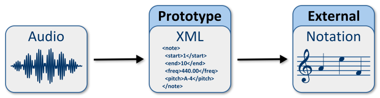
Output Model

This diagram illustrates how the prototype (the system) fits into a musician’s workflow. The XML produced by the prototype may then be notated, printed, edited, and so on in an external application; in and of itself, the output isn’t particularly pretty.
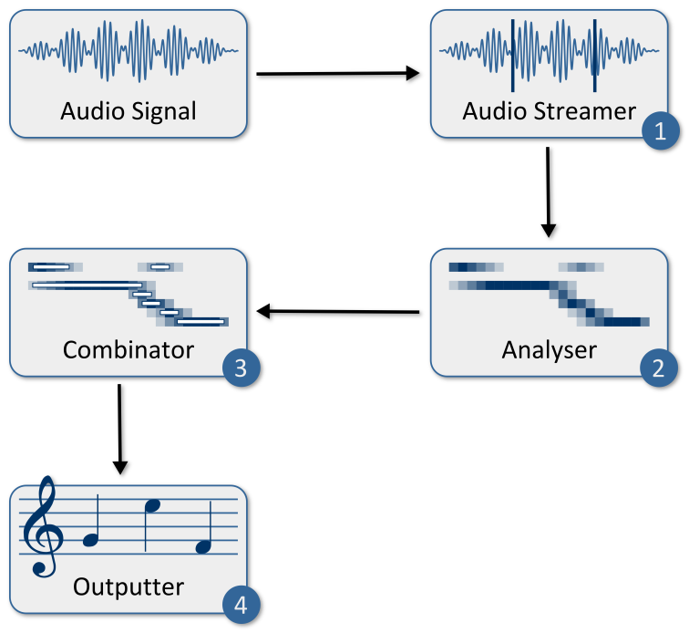
System structure

This outlines the basic underlying modular structure of the system. The Audio Streamer (1) breaks the incoming signal up into windows. It passes these windows on to the Analyser (2); this pulls frequency and amplitude information from the signal. The results of the analysis are forwarded to the Combinator (3), which is responsible for working out where actual notes are, thresholding the input, and so on. Finally, the combination results are passed to the Outputter (4), where they are converted into beautiful XML.
Window-size quantisation

Here you can see the effects of the window size on the results. The input signal (top) has notes X, Y, and Z which are 4000 samples long. The analysis, however, is being run at 6000 samples. This means that note Y falls into both of the analysis windows (with a much lower amplitude), and that the amplitudes of X and Z are detected as lower, because they only exist for two-thirds of the analysis window’s duration.
Notes

Looking at a basic sine wave, its frequency is determined by the number of complete cycles it does per second. This is measured in Hertz (Hz). The note A4 is generally agreed to have a frequency of 440Hz.
Overtones and polyphony

Musical signals are not, generally speaking, pure sine waves. They exhibit overtones, which are secondary frequencies at lower amplitudes. The ‘main’ frequency of a note is called the ‘fundamental’ frequency. Now, the difficulty is to distinguish between two different notes playing at the same time, and one note with overtones. As shown in the diagram, two notes playing at the same time (1) are added together to produce a waveform which bears little resemblence to either of its components (2). This is one of the major challenges of transcribing music automatically.
Sliding Window Analysis

Sliding window analysis is a technique used to increase temporal precision whilst maintaining accuracy in lower frequencies; remember, when using the DFT or FFT, there’s a trade-off between temporal precision (window size) and frequency accuracy (especially in the lower frequencies). It should be noted that the thesis provides the reasons for this. Anyway, sliding window analysis basically analyses the signal lots of times, using overlapping windows. In the prototype, a simple half-length sliding window analysis was used; this doubles the number of computations required, but increases accuracy significantly. It also possible to slide by a smaller amount, but for a mobile device, the computational requirements of that would just be too high.
Pyramid Analysis

An alternative method of increasing accuracy and precision is what I term “pyramid” analysis. Basically, you analyse the signal using windows of different sizes, and combine the results: large windows (1) for detecting low frequencies (with poor temporal precision), and short windows (3) for detecting high frequencies (with good temporal precision). You can also do this in a sliding window style for each window size.
Concluding remarks
Well, seeing as you’ve read this far, you deserve to be congratulated. Especially if you read the thesis, too. 😀 I hope that if you use the system, you find it useful; I may well develop it further in the not-too-distant future. I hope that some of what I said has made sense to you, and perhaps helped you to understand automated music transcription a little bit better.
All the best.